I build software with AI, and study the ideas behind it.
I’m Jubal Chandy Jacob, an AI researcher and software developer. My work spans applied AI, software development and research, with a focus on turning ideas into useful systems.
I studied Artificial Intelligence at the University of Aberdeen, where my MSc research introduced tentative landmarks for goal recognition.
Working with internal and external clients on scoping, architecture and production deployment. Building AI features with retrieval-augmented generation and domain-specific model fine-tuning.
MSc thesis · University of Aberdeen · Supervised by Dr Leonardo Amado
Goal recognition without a complete model of the environment: tentative landmarks are choke points found in example traces, and the penalised recogniser was the most accurate method on three of four benchmark domains.
Working out what an agent is trying to do from examples of its behaviour, without a complete model of its world.
MSc Artificial Intelligence dissertation · University of Aberdeen · 2026 · Supervised by Dr Leonardo Amado
The problem
Goal recognition means watching an agent act and inferring which of several goals it is pursuing, ideally before it finishes. An assistive robot, a security monitor or a conversational system all face this question: given what has happened so far, what is this agent trying to achieve?
Two families of methods dominate. Landmark-based methods use landmarks: facts or actions that must occur in every valid plan for a goal. If the agent has passed through goal A's landmarks but not goal B's, A is the better explanation. These methods are accurate and easy to explain, but finding landmarks means reasoning over every possible plan, which requires a complete, correct model of the environment and can be slow. Learning-based methods such as GRAQL learn a value function for each goal from experience. They need no model, but they lose the structure that makes landmarks explainable.
The idea: tentative landmarks
Instead of asking what every possible plan must contain, ask what every observed successful trace contains. For each goal, collect traces that reach it, keep the shortest ones, and merge them into a single graph. Any state, fact or action whose removal would disconnect the start from the goal is a tentative landmark: a choke point in the behaviour we have actually seen.
1 · Collect successful traces
2 · Merge them into one graph
3 · Find the choke points
Figure 1 Two observed traces, τ1 and τ2, are merged into one graph. Removing A or C cuts every route from I to G, so both are tentative landmarks. C is also a classical landmark, because the unseen route τ3 passes through it too. A is tentative only: τ3 bypasses it, but no observed trace did.
Whenever the traces come from valid plans, every classical landmark that appears in them is also a tentative landmark, so the idea extends classical theory rather than replacing it. The trade-off is visible in the example: a tentative landmark like A can reflect which traces happened to be sampled, rather than a true requirement of the task.
Two recognisers
hT scores each candidate goal by adding up the tentative landmarks the agent has already passed. Landmarks shared by fewer goals count for more, because they say more about which goal is being pursued.
Landmark scores have a weakness I call landmark asymmetry. Late in a long observation, wrong goals can also have many of their landmarks ticked off, so scores tie or the wrong goal wins. hTpen adds one more signal: if the agent has already taken more steps than a goal's shortest plan, that goal is a less plausible explanation. The score is divided by 1 + γ × overshoot, with γ = 0.5.
Ten observed steps against each goal's shortest planhThTpen
G1plan: 8 steps0.800.40
G2plan: 12 steps0.600.60
observed, within plan
observed, beyond the shortest plan
plan not yet observed
Figure 2 After ten observed steps, G1 leads on landmarks (0.80 vs 0.60), but its shortest plan is only eight steps long. With γ = 0.5, the two-step overshoot halves its score, and the prediction moves to G2.
Watch a run
Here is one real run from the thesis evaluation, on the Skgrid_Clean grid with the whole trace visible. The agent starts at the bottom and heads for G0, top right, but its first eight steps run along the bottom row toward G3. Watch which goal the penalised recogniser favours as each step arrives.
Figure 3 A replay of hTpen on Skgrid_Clean, problem 4. G3 leads while the agent runs along the bottom row, G2 takes over on the way up, and the true goal, G0, wins from step 15. Strict landmarks and hT end on the wrong goal. Use the controls or the arrow keys to step through it.
Results
I evaluated both recognisers on four planning benchmarks (Blocks, Hanoi, Skgrid and Skgrid_Clean), with ten problems each, against strict classical landmarks and GRAQL. The recogniser saw 10% to 100% of the agent's behaviour, and in two settings the observations included noisy detours.
Domain
GRAQL
Strict landmarks
Tentative hT
Penalised hTpen
Blocks
87.1%
77.1%
82.9%
94.3%
Hanoi
88.6%
78.6%
87.1%
92.9%
Skgrid
72.9%
42.9%
45.7%
54.3%
Skgrid_Clean
86.0%
80.0%
80.0%
90.0%
Table 1 Mean accuracy per domain, averaged over all observation levels (five clean and two noisy; Skgrid_Clean clean only). The best method in each domain is marked.
The penalised recogniser was the most accurate method on three of the four domains. GRAQL won on Skgrid, a grid with many equally short routes, where few cells are true choke points and landmarks have little to distinguish goals by. The base recogniser, hT, matched or beat strict landmarks on every domain.
Figure 4 Accuracy averaged over the four domains as more of the agent's behaviour is observed (clean observations). GRAQL leads from 30% to 70%. With the full trace, the penalised recogniser reaches 100%, while strict landmarks level off at 88%.
The penalty matters most at full observation. On Skgrid with the whole trace visible, strict landmarks and hT reach 100% accuracy only by tying the correct goal with wrong ones, so precision is 0.53. hTpen breaks those ties and raises precision to 0.91.
Tentative landmarks are also cheaper to compute, because they are found on a much smaller graph. On Blocks, extraction took 0.06 seconds compared with 79 seconds for strict landmarks, about 1,200 times faster. On the grid domains the two took about the same time.
Limits and next steps
Symmetric grids. When many equally short paths exist, few cells are true choke points. On Skgrid, hTpen reached 54.3% against GRAQL's 72.9%. Disjunctive landmarks, such as “at least one of these cells must be visited”, are the proposed fix.
Noise. The penalty relies on trace length, and noisy detours make a trace longer. At full observation, hTpen's accuracy fell from 100% to 87% once noise was added. Counting only the steps that make progress toward a goal should make the penalty robust to this.
Scope. The evaluation used a single training seed and four domains. Larger planning domains and action-only observations are the next tests.
Language as a Label: Zero-Shot Multimodal Classification of Everyday Postures under Data Scarcity
How the wording of a text prompt changes what a vision–language model sees, when there is no labelled data to train on.
MingZe Tang and Jubal Chandy Jacob · MMLoSo 2025, First Workshop on Multimodal Models for Low-Resource Contexts and Social Impact · ACL Anthology
The question
Recognising what a person is doing from a photo usually needs many labelled examples, and those are expensive to collect. Vision–language models such as CLIP offer a shortcut. They place images and text in the same space, so a sentence can act as the label: the photo is compared with one prompt per class, and the closest prompt wins.
That raises a practical question. If the sentence is the label, does describing the class in more detail help the model find it?
Photoone person, 224 × 224
Image encoderfrozen
Promptsone per class
Text encoderfrozen
Cosine similarityphoto vs. each prompt
Predictionclass of the closest prompt
Figure 1 Zero-shot classification. Each photo and each class prompt is embedded once, and nothing is trained. Only the wording of the prompts changes between experiments.
The experiment
We built a small, balanced set of 285 MS COCO photos, labelled by hand: sitting (95), standing (92), and walking or running (98). We tested three vision–language models, OpenCLIP, MetaCLIP 2 and SigLIP, and compared them with vision-only models (ViT, DINOv3) and a pose-based baseline built on YOLOv11 keypoints.
Prompt wording was the only thing that changed. Each class had one prompt at each of three tiers. No prompt mentions the scene, clothing or identity, so any difference comes from how the pose is described.
Tier 1, label: the class name in a minimal template.
Tier 2, action cue: a short phrase about what the person is doing.
Tier 3, pose geometry: the body's shape, such as the angle of the hips and knees or a vertical torso.
Tier 1 · Label
“a photo of a person standing”
Tier 2 · Action cue
“a person standing still and upright, feet planted”
Tier 3 · Pose geometry
“a person standing with legs straight and torso vertical”
Figure 2 Grad-CAM attention for one standing photo under each tier. The plain label spreads attention over the person and the background. The action cue and pose wording pull it onto the legs and feet.
What we found
More detail made the models worse. On the three-class task, every model scored highest with the plain label. Adding an action cue dropped MetaCLIP 2 from 68.8% to 55.1%, and OpenCLIP from 71.2% to 52.6%. Pose wording won some accuracy back but never beat the label. We call this prompt overfitting: extra wording narrows what the model will accept as a match.
Figure 3 Three-class zero-shot accuracy by prompt tier. Hover or use the arrow keys to read each value.
The attention maps add nuance. Detailed prompts do shift attention away from the background and onto the body, but whether that pays off depends on the model. SigLIP's overall accuracy stayed low, yet on its weakest class, walking or running, pose-geometry prompts raised its F1 score from 0.364 to 0.566 in the paper's binary task (sitting vs. walking or running).
We also trained a lightweight classifier on each model's frozen image features. Models aligned with text during pre-training gave the strongest features, though not uniformly: SigLIP ranked last. The pose-keypoint baseline came close to the best model.
Figure 4 Macro F1 on the three-class task with a classifier trained on frozen features, averaged over five runs.
What it means in practice
With little or no labelled data, start with one plain label prompt per class. It is a strong baseline.
If two similar-looking classes get confused, try a short geometric description for just those classes, and use an attribution map to check that attention has moved onto the body.
Watch the gap between the top two scores, and let the system abstain when the gap is small.
Limits
The dataset is small, uses still photos of single people and covers three postures. The prompts were hand-written in English. Results may not carry over to video, where movement over time matters, or to other languages and larger sets of actions.
Evaluation of AI Systems in Mathematics: Common Sense, Robustness, and Meta-Reasoning in LLMs
Beyond “did it get the right answer”: testing whether small maths models can ignore distractions, transfer an idea, and defend or fix their own work.
Led by Jubal Chandy Jacob, with Kalani Anderson · Team project, Evaluation of AI module, MSc Artificial Intelligence · University of Aberdeen · December 2025
The question
Maths benchmarks mostly check the final answer. Real problem solving asks for more: ignoring information that doesn't matter, recognising a familiar idea in an unfamiliar problem, and judging whether criticism of your own work is right. We asked whether three small maths models can do these things: DeepSeek-Math-7B, Phi-3.5 and Qwen2.5-Math-7B.
Three tests
1 · Red herring
2 · Conceptual fragility
3 · Socratic debugging
Figure 1 The three tests, with simplified example problems. Each checks a skill that final-answer accuracy hides: ignoring what doesn't matter, recognising a familiar idea in a new form, and handling criticism of your own work.
Red herring: 50 problems, each with an irrelevant detail added. The best response ignores it and says why.
Conceptual fragility: 15 textbook problems, each followed by a variant that needs the same insight rather than a fresh calculation.
Socratic debugging: after answering, the model is challenged to reconsider, whether its answer was right or wrong.
All three models ran locally with 4-bit quantisation, a temperature of 0 and the same step-by-step prompt. Claude Opus 4.5 graded every response against written rubrics: correctness (0–2), reasoning quality (0–3) and a meta-reasoning score (0–5) tailored to each test.
What we found
Distractors broke the explanations, not the answers. Every model's meta-reasoning score fell once a distractor was added, and the strongest model fell furthest: Qwen dropped from 4.31 to 1.74, a 60% decline. Its correctness barely moved, from 1.79 to 1.70. The models mostly filtered the distractor silently. Qwen explicitly called it irrelevant in 10% of answers; DeepSeek never did.
Figure 2 Mean meta-reasoning score (0–5) on the clean problems and on the same problems with a distractor added. The drops for Qwen and DeepSeek were statistically significant (p ≤ 0.001); Phi's was not.
Scaffolding helped. When the textbook problem came first, 73–87% of answers carried its shortcut over to the variant. DeepSeek's meta-reasoning score rose by 71% over its clean baseline. Helpful context was used well; misleading context was not rejected.
Confidence is not a signal. Challenged on a correct answer, Phi and Qwen held firm about 95% of the time, while DeepSeek gave up or wavered in more than 80% of cases. Challenged on a wrong answer, all three repeated the mistake about 90% of the time and properly fixed it in at most 7% of cases. The models react to a challenge the same way whether they are right or wrong.
Figure 3 Share of correct first answers that were strongly defended when challenged, and share of wrong first answers that were properly corrected. Phi-3.5 and Qwen are almost identical, so their lines overlap.
Why it matters
High accuracy can hide fragile reasoning. A model that cannot tell a valid criticism from simple pressure is a poor partner for tutoring or collaborative problem solving, however often its first answer is right.
Limits
The datasets are small (50 and 15 problems), only three 7B models were tested, each problem was run once, and an LLM did the grading, which can itself be wrong. The results may not hold for larger models.
Can We Recognise an AI Agent’s Wrong Goal Before It Causes Harm?
Could tentative landmarks warn us that an agent is pursuing a proxy goal, early enough to step in?
Research idea · AI safety · Goal recognition · 7 min read
An AI agent can be good at what it does and still be doing the wrong thing.
Imagine a delivery robot trained to take parcels to their intended recipients. During training, the recipient always happens to be at the blue loading bay. The robot performs well. But when the recipient moves, it continues delivering to the blue bay.
Its navigation still works. It can identify parcels, avoid obstacles and complete a delivery. What fails is the relationship between those capabilities and the objective we intended it to pursue.
Figure 1 Goal misgeneralization in the delivery example. The robot's skills transfer; its goal does not. It learned “go to the blue bay”, which was indistinguishable from “go to the recipient” during training.
This is the problem of goal misgeneralization: an agent retains its capabilities under changed conditions but behaves as though it is pursuing an unintended objective. Work by Langosco and colleagues and Shah and colleagues establishes why this can happen even when the training reward correctly specifies the desired outcome.
The research question I am exploring is whether goal recognition could help us notice this early enough to intervene.
More specifically: could tentative landmarks reveal that an agent is pursuing a proxy goal before that pursuit produces harmful consequences?
Looking at behaviour through landmarks
Goal recognition works backwards from an agent’s observed behaviour to the objectives that might explain it.
If the delivery robot picks up a particular parcel, acquires a loading-bay key and follows a particular corridor, each action provides evidence about what it might be trying to achieve. We do not need to wait until the parcel is delivered before making an inference.
Landmark-based approaches organise some of that evidence around conditions or actions that must occur on the way to a goal. For example, possessing a required key might be a landmark for reaching a locked destination. Pereira, Oren and Meneguzzi show how landmarks can support efficient goal recognition from partial observations.
Tentative landmarks relax where that necessity comes from. Instead of requiring a feature to occur in every valid plan permitted by a complete environment model, we identify features shared by a selected family of successful behaviours derived from traces.
That makes them useful when we have examples of behaviour but lack a complete symbolic model. It also makes their meaning more limited: a tentative landmark describes what appears necessary within the behaviours represented by our evidence.
My interest is whether that representation could support a practical form of agent monitoring.
The monitor might learn the same wrong lesson
There is an immediate difficulty.
If every successful delivery trace passes through the blue loading bay, a tentative-landmark recogniser might treat that bay as evidence of correct behaviour. When the robot follows the blue marker to the wrong destination, the monitor could endorse precisely the mistake it was meant to catch.
Both systems may rely on the same misleading correlation.
This leads to the central hypothesis I would like to investigate:
Tentative landmarks learned from environments in which intended goals and proxy cues vary independently may provide earlier and more reliable warnings of proxy pursuit than landmarks learned only from environments where those cues remain correlated.
For the delivery example, that means varying the recipient, destination, parcel appearance and route so that successful delivery cannot consistently be explained by “follow the blue marker.”
The idea of using distinguishing environments already has a strong precedent. Mitigating Goal Misgeneralization via Minimax Regret studies settings where intended and proxy goals usually agree during training but separate in deployment.
The distinction I want to explore is using such environments to improve an external recogniser, while keeping the monitored agent fixed. Would better evidence help the monitor identify the agent’s mistake, even when the agent itself has not been retrained?
What would “before harm” mean?
I want to keep two research aims separate:
Detection: identify behaviour consistent with proxy-goal pursuit under distribution shift.
Prevention: use that warning to intervene early enough to avoid an undesirable outcome.
Neither requires claiming that we can read an agent’s internal intentions.
There is also a limit to what behaviour can reveal. If the intended goal and a proxy predict identical observations so far, passive goal recognition cannot reliably distinguish them from that evidence alone.
The useful question is whether distinguishing evidence appears while there is still time to act.
For the robot, approaching the wrong loading bay might be recoverable. Dispatching a parcel through a one-way exit might not be. A warning after dispatch could classify the failure correctly while providing no protection.
Figure 2 Detection is only useful in the window between the moment the evidence separates the two goals and the last point where intervention can still prevent harm.
This concern appears directly in the preliminary Does Asking for Help Mitigate Goal Misgeneralization? project. Its reported results suggest that intervention strategies can look effective when agents are allowed to recover after reaching a proxy, but struggle when that outcome is irreversible. The public page currently lists its paper as forthcoming, so I treat these findings as preliminary.
Classical AI also offers an important precedent. Models of Intervention studies when an observer should intervene to avoid undesirable outcomes, including using landmark-based features.
The contribution here would therefore need to be more specific than simply combining recognition and intervention.
Starting with classical AI, then testing LLM agents
I would begin in a controlled planning environment where intended goals, proxy goals and irreversible actions can be specified clearly.
A classical planner would let us test whether the recogniser distinguishes known objectives. A learned policy in the same environment would then let us investigate misgeneralization caused by training correlations. Giving a planner the wrong objective is useful experimental control, but it does not itself demonstrate learned misgeneralization.
An LLM agent could subsequently operate through the same structured actions: inspect a parcel, select it, move, unlock a door and dispatch it. This would let us compare different kinds of agents without simultaneously changing the entire environment.
For the LLM setting, I would initially ground recognition in tool actions and verified state changes. An agent’s explanation of its intentions could be an additional source of evidence, but not ground truth.
We would also need to distinguish systematic proxy pursuit from misunderstanding, execution errors or following an injected replacement instruction. Those failures matter, but they do not all establish goal misgeneralization.
What would make the result useful?
The monitor should do more than flag unfamiliar behaviour. An unusual route may be a sensible adaptation. Conversely, familiar-looking behaviour may now serve the wrong objective.
I would therefore want to measure detection before the last safe intervention point, false alarms on valid behaviour, harmful outcomes prevented and legitimate tasks completed. Competing methods should receive the same training evidence and comparable intervention budgets.
Unknown proxies are another important test. A recogniser forced to choose among a fixed list of goals may confidently select the least-wrong explanation. It needs room to conclude that the available hypotheses do not adequately explain the behaviour.
Finally, stopping a harmful action would not establish that we had corrected the agent’s objective. It would show that the monitored system avoided a particular failure under particular conditions. That is a narrower claim, but still a useful AI safety result.
What interests me most is whether tentative landmarks can make the warning intelligible: these observations increasingly support this competing objective, and this is the point beyond which recovery becomes difficult.
I would welcome discussion from people working on planning, reinforcement learning, agent monitoring or AI safety. Where would goal recognition offer an advantage over direct safety checks—and which environments would provide the strongest test of that advantage?
References
Langosco, L., Koch, J., Sharkey, L. D., Pfau, J. and Krueger, D. (2022). Goal misgeneralization in deep reinforcement learning. Proceedings of the 39th International Conference on Machine Learning, PMLR 162, 12004–12019.
Abdel Sadek, K., Farrugia-Roberts, M., Anwar, U., Erlebach, H., Schroeder de Witt, C., Krueger, D. and Dennis, M. (2025). Mitigating goal misgeneralization via minimax regret. Reinforcement Learning Conference (RLC) 2025. arXiv:2507.03068.
A real-time pipeline where financial news sentiment drives trading decisions, built in a weekend and selected as a top finalist.
Top finalist · Hack The Burgh XII · University of Edinburgh · November 2025 · Quant finance
The challenge
Build a real-time system where market sentiment drives trading decisions. I led a core team of four, one of 30 competing teams, and we were ranked among the top finalists.
What we built
A full pipeline from live financial news to simulated trades. Headlines arrive from news APIs, are cleaned and tokenised, then scored by a DistilRoBERTa model we fine-tuned for financial news sentiment. Each bullish or bearish reading feeds a per-ticker confidence score, which a strategy engine turns into position sizes and entry timing. A trade simulator executes the signals and tracks profit and loss, drawdown and every decision.
Figure 1 The pipeline, from live news to simulated trades.
Highlights
Top finalist at Hack The Burgh XII, University of Edinburgh.
Led a team of four among 30 competing teams.
Fine-tuned DistilRoBERTa for real-time financial news sentiment.
End to end: live news, language model, bullish or bearish signal, trade simulation.
Photography
Away from code and research, I take photographs. A small selection.
Photography · Selected work
PictureIT: say it, and the picture appears
A voice-driven visual communication app for teachers, making classroom instructions, routines and stories easier for pupils to understand, including those with special educational needs and disabilities (SEND) and pupils who speak other languages.
Co-founder · EdTech startup · Web-app prototype, built for demonstration
The idea
Visual aids help pupils follow what is happening in a lesson, but finding or preparing the right one takes time a teacher rarely has mid-lesson. PictureIT keeps the visual a sentence away: a teacher says a phrase such as “take a seat” and the matching picture appears on screen. Visuals can also be found through search, favourites and categories.
Figure 1 Say it, show it. Phrases are matched against each card’s name and aliases, so “take a seat” still finds “Sit down”.
Real-time translation
Not every pupil in a class speaks the teacher’s language. With real-time translation, a teacher who speaks English can communicate with pupils who speak other languages, and they can respond, through both audio and video. Paired with the pictures, an instruction reaches a pupil in their own language and as a visual at the same time.
Figure 2 Real-time translation: the teacher speaks English, and the pupil hears and sees the instruction in their own language. Spanish is shown as an example.
What it brings together
Real-time translation. Teachers who speak English and pupils who speak other languages can understand each other, through both audio and video.
Visual resources. Custom picture cards, schedules, choice boards, emotion cards, social stories, and First–Then or Now–Next–Later boards, with AI-generated images.
Classroom presentation. Resources shown fullscreen, with optional spoken narration, voice controls and manual navigation.
Storybooks. Upload PDFs or page images, and display the relevant illustrations while reading aloud.
Reusable libraries. Save and organise cards, routines and resources for future lessons.
School administration. Manage staff, groups, shared resources, approvals and usage reports.
Figure 3 Two of the SEND resources teachers can build and present: a First–Then board and a Now–Next–Later board.
Why it matters
The aim is to reduce the time teachers spend finding or preparing visual aids, and to make those visuals available naturally during teaching. PictureIT is currently a web-app prototype, built for demonstration.
Arivu: a private assistant that understands you over time
An AI startup building a personal assistant that learns your context and keeps it on your device, starting on your Android phone.
Founder · AI startup · On-device AI · Android first
The problem
Arivu addresses two problems. You have to repeat your context in every AI conversation. And to get help that actually knows you, you have to send personal information to cloud services.
Figure 1 The two problems, and Arivu’s answer: the assistant keeps a memory of what matters to you, on your phone, so each conversation builds on the last.
Four principles
Figure 2 The four principles Arivu is being developed around.
On-device intelligence. Process conversations and personal information locally, with offline use as a core goal.
Memory with continuity. Remember relevant preferences, projects and past conversations, so each interaction builds on what came before.
Thoughtful assistance. Connect related details and ask useful follow-up questions, without making you repeat everything.
User control. Let people inspect, correct and delete memories, including seeing where each detail came from.
The memory is the heart of it. This interactive sketch from the Arivu website shows the idea: words from two messages feed through a small network, the connections they used are strengthened, and the details worth keeping form memories that link to each other over time.
Loading the sketch…
Figure 3 “Built over time”, from the Arivu website: memories form as you talk, and new ones connect to old ones. Drag to turn the network, and hover a memory to see what it was learned from. An illustration of the idea, not the product itself.
What comes next
The initial focus is an English-language assistant. The longer-term vision includes more languages and AI Mesh: a way for trusted personal devices to share tasks and selected context. Efficient models and responsible use of existing hardware guide that development.
Figure 4 AI Mesh, part of the longer-term vision: trusted personal devices share tasks and selected context with each other.
The promise
Less repetition, more understanding, and personal AI that stays yours.
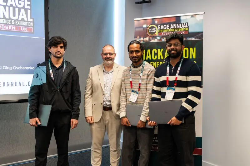
Our team, Prometheus, won with Risk-Aware Growth: a controller that grows a simulated city only as fast as its cash and power grid can safely support.
Winners · EAGE Hackathon 2026 · EAGE Annual, Aberdeen · Team Prometheus · June 2026 · Agents and energy systems
The challenge
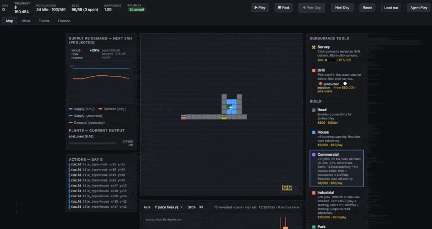
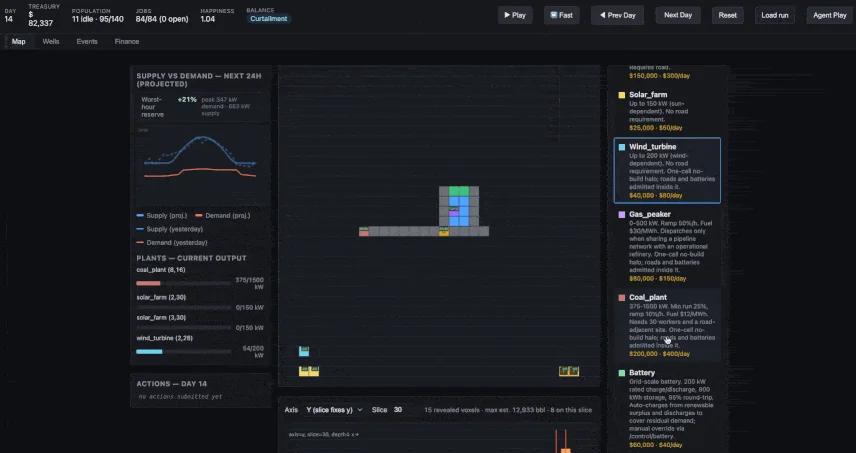
The Agent Energy Arena is a simulated city. Every simulated hour, electricity supply has to meet demand or citizens lose power; every simulated day, the books have to close in the black. An agent starts with $300,000, 100 people and one coal plant, and has to grow a profitable, populous, reasonably renewable city without going bankrupt. Teams were tested on three scenarios, including a grid-stress run (low wind and heatwaves) and an economy-stress run (fuel shock and crude-price collapse), across five random seeds.
Part of the score
Weight
Full credit
Treasury
30%
profit relative to starting cash
Population
30%
400 people
Renewable electricity
20%
50% of demand served
Happiness
10%
1.20
Solvency
10%
positive treasury every day
Table 1 How the simulator scored a run. These parts make up 85% of the score, using the whole daily history, so a strong final day cannot hide an earlier collapse. Surviving the full horizon gives the other 15%.
What we built
Risk-Aware Growth is a deterministic state machine that acts once per simulated day. It follows a fixed city plan, built in stages: housing rows, commercial blocks, parks for happiness, a second coal plant, then solar farms and batteries. It only moves to the next stage when the treasury and the grid can support it. Every stage has a minimum treasury and a cash reserve that must remain after building, and new demand is added only if the simulator’s next-day power preview is safe.
Figure 1 The controller’s daily decisions, checked in order. Under an economy shock it deliberately stops at a small, profitable city: attempts to keep growing led to debt.
What we tried first
We kept every serious approach and compared them on the same 15 cases. Stable renewable cities stayed solvent but stalled around 150 people. Oil drilling had the highest upside, with single runs near 90, but poor reservoirs or a price collapse sank it: its worst case scored 48. Learned policies (Cross-Entropy Method search and PPO) either overspent and stayed in debt or survived without growing. The lesson was that solvency had to act as a hard constraint, and that a small, checkable action space beat a clever but fragile one.
Figure 2 Median score of each approach across the 15 test cases (three scenarios × five seeds). Risk-Aware Growth was submitted.
Result
All 15 cases completed with a positive treasury every day. The median score was 89.2 and the best 89.9, on the baseline scenario, with 434 people. Under economy stress the controller stopped at a city of about 164 people by design, which kept it solvent on all five seeds.
The simulator
The Agent Energy Arena was built by Oleg Ovcharenko for the EAGE 2026 Hackathon, organised by the EAGE AI Committee, and is released under the MIT licence.
Building makemore: from counting letters to a small WaveNet
Notes from Andrej Karpathy's makemore lectures, where one small model that invents new names is rebuilt five times, each time a little closer to how modern language models work.
Lecture notes · Language models · January 2023 · 5 min read
Makemore learns from a list of 32,032 names and makes more of them. Every version does the same job: given the characters so far, predict the next one. Sampling one character at a time produces new names. What changes from part to part is how much context the model sees and how it is built. These are my notes from working through the lectures and notebooks, shortened to the ideas I keep coming back to.
1 · Counting pairs
The simplest model looks only at the previous character. Count how often each character follows each other one across all the names, with a dot marking the start and end, so “.emma.” contributes .e, em, mm, ma and a. Normalise the counts into probabilities and sample. The names that come out are poor: one character of context is not enough.
To measure quality, take the probability the model gives each character in the training names, take the log, average and negate it. This average negative log-likelihood is the loss: lower is better. The counting model scores 2.45. Adding one to every count (smoothing) stops an unseen pair from giving an infinite loss.
The same model can be trained as a tiny neural network: one-hot encode the character, apply one linear layer and a softmax, and minimise the same loss with gradient descent. It converges to the same table. The point is that the neural version can grow into something bigger; the counting version cannot.
2 · Learning character embeddings
Part two follows Bengio et al. (2003). The model looks at the last three characters, turns each into a short learned vector using one shared lookup table, and passes them through a hidden layer to a softmax over the 27 possible characters.
Figure 1 The multilayer perceptron from part two, redrawn from Bengio et al. Three characters of context go in; a probability for each of the 27 characters comes out.
The practical lessons mattered as much as the model. Train on small random batches. Find a learning rate by sweeping a range and plotting the loss. Split the names 80/10/10 into training, development and test sets: tune on the development set and touch the test set once, at the end. When training and development losses start to separate, the model is overfitting. My run reached a development loss of 2.19.
3 · Keeping activations healthy
The untrained network started with a loss far above 3.30, the value you get by guessing uniformly among 27 characters. It was confidently wrong. Shrinking the output layer's starting weights fixes that.
A subtler problem sits in the hidden layer. tanh squashes its input into −1 to 1, and inputs far from zero land on the flat ends, where the gradient is almost zero, so those neurons stop learning. Scaling the starting weights by gain ÷ √(number of inputs), with a gain of 5/3 for tanh (Kaiming initialisation), keeps inputs in the useful middle range.
Figure 2 Three common activation functions. tanh and sigmoid flatten at both ends, which is where gradients vanish.
Batch normalisation goes further: it rescales each layer's inputs over the current batch so they start out roughly standard normal, which makes deeper networks much easier to train. The catch is that it ties together the examples in a batch, a source of subtle bugs. As Karpathy puts it, “avoid it if possible”. Plots of activations, gradients and the size of each update relative to the weights became my main debugging tools. This version reached a development loss of 2.11.
4 · Backpropagation by hand
Part four replaces loss.backward() with gradients derived by hand for every step, including cross-entropy and batch normalisation. One result is worth remembering: the gradient on the logits is just the softmax probabilities, minus one at the correct character. Training pulls the wrong characters down and the right one up, and the pull stops once the right character's probability reaches one.
Forward
mean
variance
standardise
scale and shift
Backward, in the order 1 to 4
1
2
3
4
Figure 3 My batch normalisation backward pass, redrawn from my handwritten notes. The graph is the forward computation; the numbers give the order in which gradients flow back. The highlighted terms are the derivatives that take the most care. Because μ is the mean, ∂σ²/∂μ is zero, which removes a whole term.
It was hard and unintuitive at first, then suddenly clear after a few derivations. A course in calculus helps more than any shortcut.
5 · A WaveNet-style hierarchy
The MLP squashes its whole context into one layer at once. WaveNet (2016) fuses information gradually: neighbouring pairs first, then pairs of pairs, until one vector summarises the context. The lecture builds this tree with ordinary linear layers over eight characters of context. WaveNet itself computes the same tree efficiently with dilated causal convolutions.
Figure 4 Fusing eight characters of context step by step, rather than all at once.
Batch normalisation needed a fix for the new three-dimensional inputs: the statistics have to be averaged over both the batch and the position in the sequence. With that, the model reached a development loss of 1.99.
Figure 5 Loss in my runs of each notebook; lower is better. The counting model is measured on the training names; the others on held-out validation names.
What stuck with me
Most bugs are shape bugs. Broadcasting will happily do the wrong thing without an error, so check shapes as you go.
Prototype in a notebook until the shapes work, then move the code into a proper file.
Plots of activations and gradients are the debugger for neural networks.